Intro: Welcome to the E6S-Methods podcast with Jacob and Aaron, your source for expert advice on Lean, Six Sigma, and performance improvement methods. In this episode number 48, “Variations” Part 2, we conclude our introduction into various types of data distribution. Here we go.

Objection 1: These are simple terms. Everyone knows this stuff.

Counter: Perhaps. But it requires covering just to get everyone on the same page.

I Where are we going with this?

a. In order to understand Measurement System Variation, you first need an appreciation for normal variation and different types of distributions that exist

b. All sample (from process or population) variation is a combination of the tendencies of the population as well as variation tendencies of the measurement system. Measurement system variation is an artifact imposed on the sample, and thus the population as a result of trying to measure it.

II Describing a Distribution

a. Location: Central Tendency

i. Main Measures

1. Mean – Arithmetical “average” – (sum of values)/(count of values)

2. Median – The midpoint, when data is arranged in numerical order

3. Mode – most frequently occurring value (highly dependent on precision of the value)

ii. Dangers - (only tells a small part of the story)

1. Too many businesses focus on the mean of business metrics, and ignore the variation, and get a false sense of success. The customer feels the variation.

a. Two Statisticians go hunting. To better their chances, they shoot at the same time. One misses 10 feet to the left, the other misses 10 feet to the right. They stand and high-five each-other, knowing “on average” they made the kill.

b. Put your head in and oven, and your feet in a freezer. On average your temperature is normal

b. Spread

i. Main Measures

1. Standard Deviation – The “average” distance each point is from the mean (geometrical average)

2. Variance – Square of Standard Deviation

3. Range – Difference between the maximum value and the minimum value

ii. Dangers – Most meaningful when combined with a location measurement (i.e. mean)

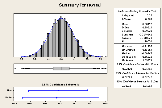
c. Histograms & Shapes – Less dangerous if ignored. Often assume Normal, symmetrical distribution. Knowing the shape of the distribution is helpful when trying to get a more advanced understanding or process or population behavior.

i. Symetrical – Mirror image from the center

ii. Skewed – Shifted to one side. Non-symmetrical.

1. “Positive Skew” or “Skewed Right” – “Head” to left, & “Tail” to far right

2. “Negative Skew” or “Skewed Left” – “Head to right, & “Tail” to far left

http://en.wikipedia.org/wiki/Skewness

iii. Multi-Modal – More than one mode. (Many humps)

1. Bimodal

iv. Truncated – Cut short. Can look like a normal distribution that is “trimmed” or cut off at a single value. (in certain circumstances this may indicate poor integrity in reporting data, when the distribution truncates right at the specification limit.)

v. Some Additional Shape Terms

1. Skewness: Degree of shift from symmetry

a. Basic Definition: (Mean-Median)/(Sigma). Closer to zero, more symmetrical. If negative value, then Median>Mean, and equals “Negative Skew” (Tail Left)

2. Kurtosis: “Sharpness” of the peak. A high kurtosis distribution has a sharper peak and fatter tails, while a low kurtosis distribution has a more rounded peak and thinner tails.

a. Normal Curve is in the middle. Uniform (flat) Distribution has a negative kurtosis value. Sharper peaks, like Exponential Distributions have high positive kurtosis.

III What if I don’t have fancy software?

a. You can estimate normality by how close mean, median & mode are to one another. If they are close, you may assume you can approximate using “normal” statistics. (You should at least have MS Excel if you’re dealing with large data sets.)

b. key tips for estimating normality; how measurement variation fits in.

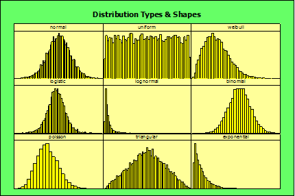
IV Some Standard Distributions:

a. Single Mode Symmetrical

i. Normal (Focus of most LSS Projects), Logistic, Binomial, Triangular….

b. Skewed

i. Weibull (Life Testing, Warranty, etc) Lognormal, Poisson, Exponential…

c. Flat:

i. Uniform : Rolling a Single Die (Dice): Each value has equal probability of being chosen.

a. In order to understand Measurement System Variation, you first need an appreciation for normal variation and different types of distributions that exist

V Where are we going with this?

a. In order to understand Measurement System Variation, you first need an appreciation for normal variation and different types of distributions that exist

Outro: Thanks for listening to episode 48 of the E6S-Methods Podcast. Stay tuned for episode number 49 where we kick off our series on Measurement System Variation. This is your chance to “Rule out the Ruler.” Subscribe to past and future episodes on iTunes or stream us live on-demand with Stitcher Radio. Have an idea for an episode? Contact us! Follow us on twitter @e6sindustries. Join a discussion on LinkedIn. Find outlines and graphics for all shows and more at www.E6S-Methods.com. “Journey Through Success”